Powell River Project - Passive Treatment of Acid-Mine Drainage

Introduction

Acidic mine drainage (AMD; also called “acid rock drainage” or “acid drainage”) is an environmental pollutant that impairs water resources in mining regions throughout the world. Where such treatment is required legally, treatment must be efficient and continual. Treatment methods are commonly divided into either “active,” meaning reliance on the addition of alkaline chemicals to neutralize the acidity, or “passive.” The term “passive treatment” means reliance on biological, geochemical, and gravitational processes. Passive treatment does not require constant care or the chemical reagents that characterize “active” AMD treatment.

This publication presents guidance for design of passive treatment systems for AMD. Our emphasis is to describe clearly the mechanisms governing these systems’ treatment effectiveness and performance. Parties intending to construct passive treatment systems may refer to other sources that include more detailed design and construction guidance, including those listed as “Design Guidelines” in the references below. Articles by Skousen and Ziemkiewicz (2005), and Skousen (1996), contain photographs that illustrate many of these concepts.

Acid Mine Drainage

Acid drainage occurs when minerals containing reduced forms of sulfur (S) oxidize via exposure to oxygen and water during earth disturbances (Figure 1). In coalmining areas, the most common of these minerals is iron pyrite (FeS₂). Using FeS₂ as an example, AMD formation can be represented as follows:

FeS₂(s) + 3.5 O₂ + H₂O → Fe⁺² + 2 SO₄^-2 + H⁺ (eq. 1)

Fe⁺² + 0.25 O₂ + H⁺ → Fe⁺³ + 0.5 H₂O (eq. 2)

Fe⁺³ + 2 H₂O → FeOOH (s) + 3 H⁺ (eq. 3)

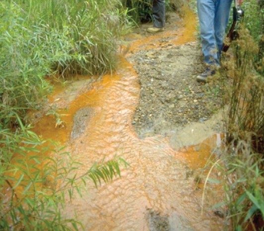
The process is initiated with pyrite oxidation and release of ferrous iron (Fe⁺²), sulfate (SO₄^2-), and hydrogen (H⁺) (eq. 1). The sulfur-oxidation process is accelerated by the presence of Thiobacillus and Ferroplasma bacteria. Ferrous iron undergoes oxidation forming ferric iron (Fe⁺³) (eq. 2). Finally, Fe⁺³ is hydrolyzed (reacts with H₂O) to form ferric hydroxide (FeOOH), an insoluble orange-colored precipitant, and release additional acidity (eq. 3). The rate of FeOOH formation is pH-dependent; it occurs rapidly when pH > 4.

While most of the acid drainage in the Appalachian region occurs with pyrites associated with coals, many metals other than Fe occur as reduced-S mineral forms. Many ores that are mined and processed to produce metals occur as reduced-S mineral forms (e.g., CdS, CuS, HgS, NiS, PbS, ZnS); therefore, acid mine drainage is associated with both coal and non-coal mining, and the FeS₂ oxidation process described above is illustrative of a more general process of reduced-S-mineral oxidation which releases SO₄^2- , H+, and associated metals.

Acid drainage can have dramatic impact on water quality. When large quantities of reduced-S mineral are exposed to air and water, large quantities of H+ are released causing very low water pH – sometimes < 3. Generally, the extreme acidity mobilizes (produces soluble forms which are carried by drainage waters) metals that are released from the sulfide minerals that oxidize and from associated minerals. This mobilization occurs because a number of metals – including Al, Cu, Fe, Hg, Ni, Pb, Zn – become more soluble in water as pH declines and are said to be “acid soluble.” Acid drainage also produces waters that contain high concentrations of dissolved mineral salts (“total dissolved solids,” or TDS), including the sulfates produced by mineral oxidation, mobilized acid-soluble metals, and other mineral components that become soluble due to mineral dissolution caused by the extreme acidity. In sum: acid drainage is an acidic, sulfate rich, high TDS, metal-bearing solution that harms stream ecology.

Acidity and Alkalinity

In this bulletin, passive system performance measures are expressed as removal of acidity from the treatment waters. Acidity is a measure a solution’s capacity to neutralize additions of an alkaline reagent, such as NaOH. One way to determine acidity is to add NaOH to the solution in an amount sufficient to raise pH to 8.3; the amount of acid-neutralization (OH^-) added is converted to an equivalent acidity concentration. In acid-drainage treatment, the water’s acidity is an indicator of the amount of treatment that must be applied to neutralize both the H⁺ present in solution (the solution pH), and the H⁺ that will be generated as soluble metals oxidize and/or hydrolyze, and precipitate. Acidity is usually expressed on a CaCO₃-equivalent basis, recognizing that 50 mg of CaCO₃ can neutralize 1 mg of H⁺.

Fe in solution is a source of acidity because the chemical reactions that cause it to change from liquid to solid phase (to precipitate) and removed from solution release H⁺ (see equation 3). Similarly, soluble Al also contributes to acidity because it hydrolyzes as OH^- ions are added and pH is raised; Al eventually precipitates as a solid-phase chemical form, releasing H⁺ in the process:

Al⁺³ + 3 H₂O → Al(OH)₃ (s) + 3 H⁺ (eq. 4)

Another common source of acidity in mine drainage is Mn. There are several pathways by which Mn can be neutralized, all of which generate H⁺, including that represented below which occurs when O2 is present:

Mn²⁺ + 0.25 O₂ + 1.5 H₂O → MnOOH (s) + 2H⁺ (eq. 5)

Like the FeOOH formation reaction described above (eq. 3), Mn precipitation reaction rates are influenced by pH and occur more rapidly as pH is raised, but Mn precipitation generally occurs more slowly and requires higher solution pH’s than other metals. The presence of acid-soluble metals such as Fe, Al, and Mn also tends to hinder, or buffer, changes in pH that would otherwise occur in response to OH- additions because their precipitation generates additional H⁺.

If a solution’s chemistry is known, acidity can be estimated using an equation that considers the molecular weight of each acid-soluble metal in solution at an environmentally significant concentration, the number of protons (H⁺) to be generated per mole as those metals precipitate, and the solution pH. A commonly used form of that equation is as follows:

A = 50*[ 2*(Fe⁺²/56) + 3*(Fe⁺³/56) + 2*(Mn/55) + 3*(Al/27) + 1000*(10^-pH)] (eq. 6)

In this equation, A = Acidity, expressed as mg/L CaCO3 equivalent (50 is the initial multiplication factor because 50 mg of CaCO3 can neutralize 1 mg of H+); and Fe+2, Fe+3, Mn, and Al are concentrations in solution, as mg/L. When other acid-soluble metals are present in known concentrations (Zn, Cu, Ni, etc.), similar terms are added to the equation to estimate the acidity contributions by these other metals. The acidity calculated using equation 6 is an estimate of the true acidity, because acid-soluble metals can react along several reaction paths, depending on solution chemistry. However, several studies (Watzlaf et al. 2004, Kirby and Cravotta 2005) demonstrate that calculated acidities are generally close to measured acidities for acid drainage solutions collected from the Appalachian coalfields, and that pH alone is generally a poor estimator for acidity.

A solution’s alkalinity is measured by titrating with a strong acid, usually H₂SO₄, to pH of 4.5. Thus, a solution with pH > 4.5 but < 7 can have both alkalinity and acidity. In this bulletin, the term “alkalinity” is used generally to describe a solution’s potential to neutralize acidity. The net acidity of a solution can be determined by subtracting measured alkalinity from measured or calculated acidity; and the net alkalinity can be determined by subtracting acidity from alkalinity. See Kirby and Cravotta (2005) for a thorough review of acidity and alkalinity. Throughout this bulletin, acidity and alkalinity concentrations are expressed on a CaCO₃-equivalent basis.

Passive Treatment of AMD

Passive treatment systems for acid drainage are intended to renovate and improve the quality of waters that pass through them. These systems are modeled after wetlands and other natural processes, with modifications directed toward meeting specific treatment goals. Early research included investigations of natural wetlands that were receiving AMD (Weider and Lang 1982) that raised pH and reduced Fe concentrations without visible deterioration.

A critical step in designing passive treatment is to characterize the waters to be treated. This can be done by measuring the discharge or flow of those waters and the concentrations of water-quality constituents of concern over an extended period–ideally at least a year—to determine how these quantities vary seasonally. Based on this information plus knowledge of the system’s purpose (whether it will stand alone or be used in combination with another treatment process, or is intended for regulatory compliance), the elemental concentrations and flow volume to be treated are determined – these are the “design conditions.” Site characteristics, especially land availability, also influence passive treatment system selection and design.

Aerobic Wetlands

Aerobic wetlands are the simplest type of passive treatment system but are limited in the types of waters they can treat effectively. Aerobic wetlands are used to treat mildly acidic or net-alkaline waters containing elevated Fe concentrations. They have limited capacity to neutralize acidity. These systems’ primary function is to allow aeration to the mine waters flowing among the vegetation, allowing dissolved Fe to oxidize, and to provide residence time where the water is slowed for Fe oxide products to precipitate. Because Fe precipitation generates H⁺, the water leaving the aerobic wetland may be lower in pH than that entering, even if Fe concentrations are less.

Where influent waters are net-alkaline and Fe is not in solution at significant concentrations, aerobic wetlands are also capable of removing manganese (Mn). However, Mn-removal effectiveness is limited by several factors. Mn removal occurs via mechanisms similar to the removal of Fe, but more slowly. Dissolved Mn can oxidize to solid-phase forms, such as MnO₂ (manganese dioxide), but the process is very slow when pH < 8 and, like Fe oxidation, it generates acidity. As with Fe, Mn oxidation occurs both chemically and microbially. However, Fe oxidation is a preferential process so Mn oxidation does not occur as a significant process until Fe oxidation is nearly complete. For aerobic wetlands to remove Mn successfully, large areas or additional wetland cells are required.
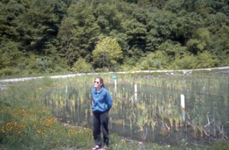
A typical aerobic wetland system is a shallow, surface-flow wetland planted with cattails (Typha sp.) (Figure 2). The depression that holds the wetland may or may not be lined with a synthetic or clay barrier. Depending on landscape conditions, the lining can be intended to either to keep treatment waters from draining out through the depression’s base or to prevent environmental waters from moving into the system and thus diluting the waters to be treated.

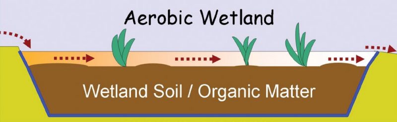
Substrates vary from natural soils to composted organic matter. Shallow water levels (10-30 cm) are generally maintained for the aerobic conditions and to enable growth of aquatic plants which aid wetland performance. Constructing the system with variable water depths within the 10-30 cm range encourages plant community diversity. Plants serve as physical obstacles which help to prevent “channelized flow,” a condition that occurs when flowing waters are concentrated within the shortest distance between the entrance and exit; thus, plants can help to disperse water flows throughout the wetland for more effective treatment. Dispersed flow causes the waters to move more slowly, allowing more time for the oxidation and aiding in physical filtration and sedimentation of small particles. Species such as cattails translocate O₂ from the atmosphere through their roots, which also aids oxidation. Although most aquatic plants will remove some metals from the water column, their capacity is quite limited relative to overall metal loadings that these systems usually receive. Therefore, metal uptake by plants plays only a minor role in water treatment by these systems.

Aerobic wetlands are often designed in series with a small sedimentation basin that contains no plants. Waters to be treated may flow through the sedimentation basin prior to entering the aerobic wetland which allows suspended sediments and easily hydrolyzable Fe+3 to settle out, The pre-treatment basin is designed to extend the aerobic wetland’s useful life by accumulating particles that would otherwise settle in the wetland system.

Commonly cited design criteria are based on the total surface area required to treat anticipated Fe and Mn loadings (Table 1). Because performance varies with factors such as weather and streamflow, more conservative design criteria are recommended when systems are intended to achieve regulatory compliance because the penalties for even occasional failure to perform as expected can be significant.

Data from Skousen and Ziemkiewicz (2005) demonstrate that aerobic wetland treatment systems do not always perform in an equivalent manner to the design criteria (Figure 3). On a total acidity basis, the design criteria for non-regulatory compliance (20 g/m2/ day of Fe) is equivalent to about 36 g/m2/day of total acidity, assuming that most of the soluble iron is in the Fe⁺² form, which would be expected at pH = ~7. For non-regulatory compliance purposes, Fe-based design criteria would be roughly half that level (meaning that the wetland as designed to be twice as large). The aerobic wetland systems demonstrate variable performance, with only 2 of the 6 performing within the range of design criteria for regulatory compliance and 2 additional approximating non-regulatory compliance criteria.

Modifications of the aerobic wetland design allow these systems to add alkalinity and effectively treat net acid waters (Figure 4). These include the addition of a bed of limestone beneath or mixed with an organic substrate, which encourages generation of alkalinity as bicarbonate (HCO_4-). Sulfate reduction is a microbial process that occurs under anoxic (low O₂) conditions when sulfates and biodegradable organics are present. Sulfate-reducing bacteria utilize the O that enters the anoxic environment as a component of sulfate (SO₄^2-) for metabolic processing of biodegradable organics, transforming the associated S to either hydrogen sulfide gas (H₂S) or to a solid-phase sulfide. The most common form of sulfide reduction generates H₂S and bicarbonate alkalinity:

SO₄^-2 + 2 CH₂O → H₂S + 2 HCO₃- (eq. 7)

Sulfate reduction is common in both natural and treatment wetlands where its occurrence can often be detected as visible bubbles emerging from the substrate accompanied by the “rotten egg” odor of H₂S gas. When acid-soluble metals are in solution, sulfate reduction can form solid-phase metal sulfides as an alternative end product, which removes metals from solution and deposits them in the substrate. In the following, “M” represents a sulfide-forming metal and “MS” represents a metal sulfide.

M+ SO₄^-2 + CH₂O → MS + HCO₃ - (eq. 8)

The other alkalinity generating process is dissolution of the limestone within or below the organic substrate:

CaCO₃ + H⁺ → Ca²⁺ + HCO₃^- (eq. 9)

The bicarbonate (HCO₃-) is a source of alkalinity, and can neutralize H+ and/or raise pH to enhance precipitation of acid-soluble metals:

HCO₃^- + H⁺ → H₂O + CO₂ (aq) (eq. 10)

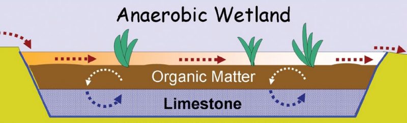
High-Ca limestones, with greater than 90% CaCO₃, are preferred for passive treatment use because they are more soluble than impure limestones or those that contain a larger proportion of total carbonates as MgCO₃ (dolomitic limestones). The limestone is placed so that waters must move through organic substrate prior to contacting it, which allows bacteria in the organic material to remove O₂ from the percolating waters. This process helps to prevent armoring of the limestone. The term “armoring” refers to coating of Fe on limestone surfaces, a process that renders those surfaces less reactive.

Anaerobic wetlands are capable of removing acid-soluble metals, especially Fe and Al, and producing alkalinity. However, their effectiveness is limited by the slow mixing of the alkaline substrate water with acidic waters near the surface. Thus, these systems commonly require large surface areas and long retention times. Like other passive treatment systems, their effectiveness at removing Mn is limited unless very large areas are used.

Research reported by Skousen demonstrates that substrate processes – alkalinity generation to stimulate oxidation and hydrolysis, and metal sulfide formation– are the primary drivers of water quality renovation over the long term. When the systems are first constructed, mechanisms such as plant uptake and sorption by organic materials can contribute to metal removal, but the capacity of these mechanisms to remove metals is soon exhausted as absorption sites are filled.

General guidelines for anaerobic wetland construction advocate use of a 30–60 cm layer of organic matter over 15–30 cm bed of limestone, or placing a mixture of organic matter and limestone to a depth of 50–100 cm. The organic matter must be water permeable and biodegradable. Materials such as spent mushroom compost have been used successfully at a number of sites in northern Appalachia. Cattails (Typha sp.) or other aquatic vegetation may be planted throughout the wetland to supply additional organic matter for the O₂-consuming bacteria and to promote metal oxidation with the release of oxygen from their root system. If sediments or easily hydrolysable Fe are present in the waters to be treated, a pretreatment pond can be included in the system design.

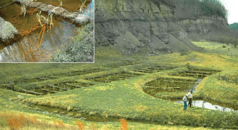
The design depth of water over the organic/limestone mixture varies. Some anaerobic wetland designs maintain water depths of 10–30 cm to encourage aquatic vegetation that prevents flow channelization and adds fresh organic material to the substrate. Other designers use deeper waters and do not encourage vegetation, reasoning that the translocation of oxygen to substrates through the roots of species, such as cattails, hinders substrate functions which are critical to performance and require anoxic conditions. When plants are not present, physical barriers can be installed to prevent flow channelization and additional organic materials can be added manually (Figure 5).

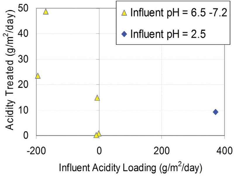
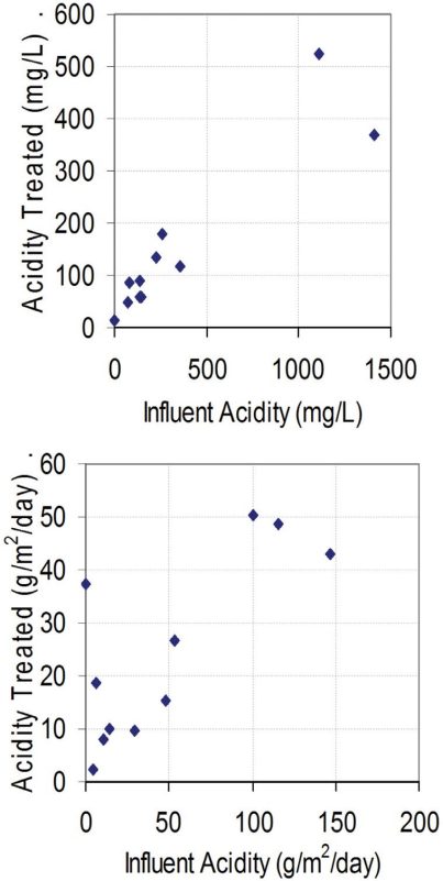
Available guidelines for system sizing recommend planning for acidity removal rates of 3.5 g/m2/day when the system is intended for regulatory compliance and 7 g/m2/day otherwise. However, performance data (Skousen and Ziemkiewicz 2005; Figure 6) demonstrate that anaerobic wetland performance is highly variable and that these systems tend to neutralize acidity more effectively when receiving higher influent acidity concentrations and loadings. Of the 16 systems whose performance was documented, eight were removing acidity at rates of ~10 g/m2/day or greater.

Anoxic Limestone Drains

Anoxic limestone drains (ALDs) can also be used to treat acidic waters (Figure 7). ALDs are limestone-filled trenches through which acidic water is directed so the limestone can produce bicarbonate alkalinity via dissolution (eq. 9). ALDs are capped with clay or compacted soil to prevent AMD contact with oxygen. The effluent is held in a settling pond to allow pH adjustment and metal precipitation prior to being discharged to natural water courses. Where water quality is suitable for an ALD, an ALD can be used to pretreat the AMD prior to forcing the waters through subsequent passive treatment units.

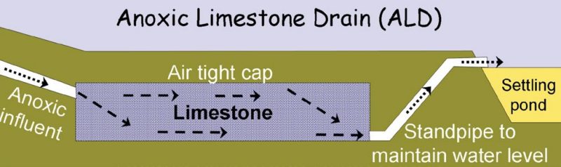
When working as intended, ALDs can renovate acidic waters more cost effectively than wetland-based systems. ALDs, however, are not capable of treating all AMD waters. Significant concentrations of O₂, Al or Fe+3 in the water will cause an ALD to clog with metal-hydroxides once a pH of 4.5 or above is reached. When excess Fe⁺³ is present in the AMD or is allowed to form from Fe⁺² due to the presence of O₂, solid-phase Fe can precipitate within the ALD (eq. 3), while Al precipitation can occur as pH increases even when O2 is excluded (eq. 4). If significant metal precipitation occurs within the ALD, the precipitant floc (a gel comprised of hydrolyzed solid-phase metal precipitants) clogs the ALD’s pores, hindering the waters from moving through the system and impairing its function. Once an ALD becomes clogged with precipitants, it becomes non-functional and must be replaced, repaired, or abandoned.

To maximize the probability that an ALD will not clog, Fe⁺³, Al, and dissolved O concentrations of the influent waters should all be below 1 mg/L. However, Skousen and others (2000) recommend that ALDs can be used successfully for AMD with dissolved O2 concentrations of up to 2 mg/L and Al concentrations of up to 25 mg/L, when less than 10 percent of total Fe in the Fe⁺³ form. Although such ALDs can be expected to clog eventually, they can still offer cost-effective water treatment compared to other passive system processes during their time of operation. ALDs are far less costly to construct than anaerobic or vertical flow wetland treatment systems and can render less costly treatment on a lifecycle basis, even if periodic but infrequent repair and replacement is required.

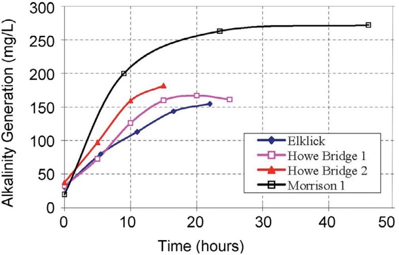
The term “retention time” means the amount of time the average quantity of water flowing through the drain spends within the drain structure, and is calculated as [total pore volume]/[Average Rate of Flow Through the Drain]. A common recommended design criterion is that ALDs should achieve at least 15 hour retention times. This criterion is based on research conducted by Watzlaf and others (2000) who established series of sampling ports in several ALDs; they were able to withdraw water samples at several points so as to observe how water quality changed as it moved through the ALDs. They observed that alkalinity generation reached maximum levels, which was within the range of 150– 300 mg/L (as CaCO₃) after 14 to 23 hours retention time. As dissolved Ca⁺² and HCO_3- concentrations approached saturation, continued limestone dissolution and alkalinity generation was hindered (Figure 8). As a result, standard design guidelines for ALDs generally recommend that drains be constructed to achieve 15 hour retention times over their design lifetimes. Limestone will most likely dissolve over that lifetime, so the initial construction achieves a longer retention time. An equation that is commonly used in ALD design is as follows:

M = [Q * ρ * t / V] + [Q * C * T / x] (eq. 10)

In this equation, M represents the mass of limestone to be used to construct the drain. The first bracketed term represents the volume of limestone required to achieve the design retention time, while the second bracketed term represents the volume of limestone expected to dissolve over the design lifetime. Adding the two quantities is intended to assure that the mass of limestone remaining in the drain throughout its design lifetime is adequate to achieve the design retention time. To calculate the first bracketed term: Q = water flow rate; ρ = limestone density; t = design retention time; and V = bulk void volume of the limestone gravel, expressed as a percent of total volume. To calculate the second bracketed term: Q = influent flow rate; C = expected rate of alkalinity generation, expressed on an mg- CaCO₃/L per unit time basis; T = the design lifetime; and x = the CaCO₃ content of the limestone, for which 90% or greater is recommended.

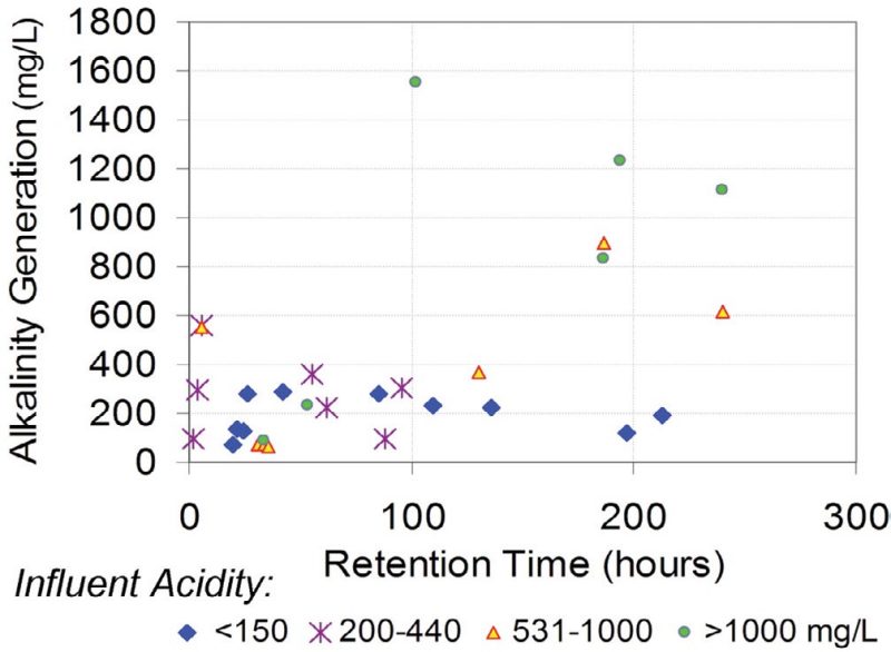
ALD performance data compiled by Skousen and Ziemkiewicz (2005) demonstrates that, like other passive treatment system, ALD performance is highly variable (Figure 9). Twenty of the 36 ALDs had estimated average influent acidities of 440 mg/L or less, close to the range of systems used to generate the 15-hour retention time design guideline. All generated alkalinities of 400 mg/L or less, and most were close to or within the 150 to 300 mg/L alkalinity target range. However, 14 of the ALDs documented were treating waters with influent acidities of 591 mg/L or greater, and most of these systems were generating alkalinities considerably above the commonly cited 150-to-300 mg/L target range; among this group, those with longer retention times tended to generate the most alkalinity.

Open Limestone Channels

An open-air analog to the ALD is the open limestone channel (OLC). These systems are employed where AMD must be conveyed over some distance prior to or during treatment. OLCs are simple to construct and operate, if the terrain is favorable: an open channel conveying the AMD is lined with high-Ca limestone. Even though the limestone typically becomes armored with Fe, the armored limestone retains some treatment effectiveness. OLCs are most effective when placed on slopes of greater than 20 percent or when they receive periodic high flows, as the abrasive action of fast-moving water and suspended particles tends to dislodge the Fe armoring, refreshing the surface for treatment effectiveness. OLCs can be effective as one element of a passive treatment system (Figure 10), but typically are not relied upon for stand-alone AMD treatment (Ziemkiewicz et al. 1997; Skousen, Sexstone, and Ziemkiwicz 2000).

Vertical Flow Systems

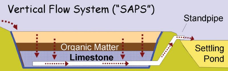
Vertical flow passive-treatment systems combine the treatment mechanisms of anaerobic wetlands and ALDs in an attempt to compensate for the limitations of both (Hendricks 1991; Duddleston et al. 1992; Kepler and McCleary 1994) (Figure 11). Vertical-flow systems have also been called SAPS (for “successive alkalinity producing systems,” Kepler and McCleary 1994) and RAPS (for “reducing and alkalinity producing systems,” Watzlaf et al. 2000).

The basic elements of these systems are similar to the anaerobic wetland, but a drainage system is added to force the AMD into direct contact with the alkalinity-producing substrate. The three major system elements are the drainage system, a limestone layer, and an organic layer (Figure 12). The system is constructed within a water-tight basin, and the drainage system is constructed with a standpipe to control water depths and ensure that the organic and limestone layers remain submerged. As the AMD waters flow downward through the organic layer, essential functions are performed: dissolved oxygen is removed by aerobic bacteria utilizing biodegradable organic compounds as energy sources, and sulfate-reducing bacteria generate alkalinity and sequester metals as sulfides (eq. 7-9). An organic layer capable of lowering DO concentrations to < 1 mg/L is essential to prevent limestone armoring and for sulfate reduction. In the limestone layer, CaCO₃ is dissolved by the acidic, anoxic waters moving down to the drainage system, producing additional alkalinity. The final effluent is discharged into a settling pond for acid neutralization and metal precipitation prior to ultimate discharge. For influents containing significant quantities of Fe⁺³ and/or sediment, vertical-flow systems should be preceded by either a settling pond or an aerobic wetland so as to limit accumulation of solids on the organic layer surface. For treating highly acidic discharges, several vertical flow cells can be placed in sequence, separated by settling ponds.

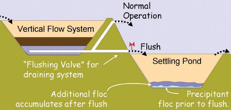
Two major limitations to the long term performance of vertical flow systems are accumulation of metal floc, primarily Fe and Al in the limestone layer, and degradation of the organic layer. In order to postpone floc accumulation and eventual clogging, a valved flushing pipe is typically included as a part of the drainage system (Kepler and McCleary 1997; Figure 13). When opened, this valved drain discharges at a lower elevation than the standpipe. Head pressure moves waters through the system rapidly, flushing the gel-like flocs of Al and Fe (“floc”) that tend to accumulate in the drainage pipes and limestone pores. Opening this valve periodically is intended to remove loose floc from the limestone layer, discharging it into the settling pond. In order to assure adequate head pressure for flushing, water depths above the organic layer of 1 to 2 m or greater are generally recommended. However, as demonstrated by Watzlaf, Kairies, and Schroeder (2002), only a small proportion of the total accumulated floc is removed by typical flushing operations. Because floc accumulates within the limestone layer, many vertical flow systems are designed with intricate drainage configurations to aid floc removal by the flushing operation.

Generally, systems are built with high-calcium (> 90%) limestone in the 4-to-6 inch size range with a limestone layer thickness in the range of 60 to 100 cm. In order to assure that the volume of limestone is adequate to assure long-term performance, the criteria used to size ALDs (eq. 10) can also be applied to calculate a volume of limestone.

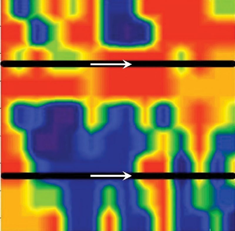
The organic layer is the other major system element that is critical to long-term performance. To operate properly, the organic layer must be sufficiently biodegradable to allow essential functions – but it also must be permeable, so water can move through it into the limestone. Organic functionality can be expected to degrade over time, due to microbial biodegradation and floc accumulation in pore spaces. Materials that have been used successfully include spent mushroom compost, composted manure, and mixtures of composted materials with less-expensive organic sources such as rotting hay. Published design guidelines recommend organic layer depths of 15–60 cm. Carefully install the organic layer to assure that the material is well mixed and applied at a uniform depth across the limestone-layer surface. Once the organic layer is in place, any activity causing compaction or physical disturbance should be avoided to prevent creation of zones of preferential vertical flow that that will “short circuit” the system and decrease treatment effectiveness (Figure 14).

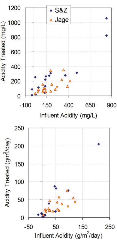
Vertical flow systems can neutralize acidity and promote metal precipitation in difficult treatment situations. Due to the forced contact of the AMD with the limestone, acid neutralization is more rapid in vertical flow systems than in anaerobic wetlands, so vertical-flow systems generally require shorter residence times and smaller surface areas. Skousen and Ziemkiewicz (2005) describe a system design guideline that sizes vertical flow systems to treat 20 g/m²/day with a 15-hour retention time, assuming the system can attain a 20-year useful life. As a general guideline, Watzlaf et al. (2004) recommend that the initial vertical-flow cell in a sequence can be sized assuming it will generate 40–60 g/m²/day of alkalinity, and that subsequent cells can be expected to generate 15–20 g/m²/day. Analysis of performance data gathered by Skousen and Ziemkiewicz (2005) and by Jage, Zipper, and Noble (2001) demonstrate that influent acidity concentrations and loadings influence performance (Figure 15). Of the 33 vertical-flow systems whose performance was documented by two studies, 19 generated alkalinity at > 20 g/m²/day and 13 generated alkalinity at > 40 g/m2/ day. Generally, systems receiving higher acid loadings generated more alkalinity, on both a concentration and a per unit surface area basis, than those receiving lower loadings.

Jage et al. (2001) have described a more detailed system for vertical flow system sizing. Their guidelines are based on the observation that the primary factor governing alkalinity generation is the rate at which limestone dissolves, which is affected by solution chemistry. Residence time in the limestone layer is one factor governing the limestone dissolution rate, as limestone can be expected to dissolve most rapidly during the first few hours of AMD contact. As the waters in contact with the limestone become saturated with dissolved Ca²⁺ and HCO₃^-, the rate of limestone dissolution slows considerably. Another factor governing the rate at which limestone dissolves is pH; at lower pH’s, CaCO₃ dissolves more rapidly. Based on these observations, they defined a method for sizing the limestone layer of a vertical flow system. The first step is to calculate a quantity which they termed as non-manganese acidity (NMA) for the influent waters:

NMA = A - 100 * Mn / 55 (eq. 11)

where A = acidity (mg/L as CaCO₃) and Mn = Mn concentration (mg/L) of the influent waters; NMA = non- Mn acidity, that component of acidity derived from H⁺ and from Al and Fe, expressed as mg/L CaCO₃. In other words, NMA is total acidity, as estimated using equation 6, minus its Mn-derived component. The rationale for using NMA as a basis for sizing is that Mn is not removed effectively by most vertical flow systems because its rapid oxidation requires pH be greater than the practical maximum (from pH 7.0 to 7.5) that most passive treatment systems are able to achieve. This practical maximum occurs because CaCO₃ dissolution rates decline as solutions become increasingly alkaline.

Once the design rate of alkalinity generation has been determined, the limestone residence time can be estimated using the equation below:

Alk = 99.3 * log 10(tr) + 0.76 * Fe + 0.23 * NMA - 58.02 (eq. 12)

where Alk = alkalinity to be generated (mg/L as CaCO3); Fe = total iron concentration (mg/L) of the design influent water quality, NMA is as in equation 11, and tr = average residence time in the limestone layer expressed in hours.

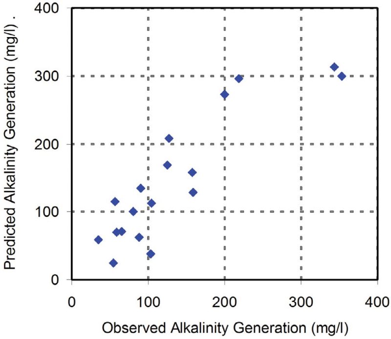
Equation 12 was developed by analyzing data from 18 vertical flow systems receiving influent waters with Fe < 300 mg/L, Al < 60 mg/L, and NMA < 500 mg/L (Jage et al. 2001). Equation 12 is not expected or intended to give precise results, but it can be used to provide design guidance. Figure 15 shows the relationship of observed alkalinity generation, averaged over periods exceeding one year, to equation 12 predictions for 18 vertical flow cells at 5 locations. All values plotted are system averages over periods exceeding one year.

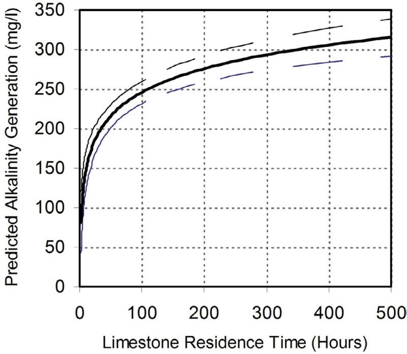
Equation 12 can be applied to illustrate the logic for constructing several vertical flow systems in series, separated by settling ponds, as an alternative to construction of a single large system. Consider a discharge with Fe = 60 mg/l, Mn = 20 mg/l, and total acidity = 300 mg/l as CaCO3 (Figure 17). Equation 12 predicts that a limestone residence time on the order of 350 hours would be required in a single cell to generate 300 mg/L acidity as needed to neutralize 260 mg/L of influent non-Mn acidity. As an alternative, construction of two cells in series, each with a 15-hour residence time and separated by a settling pond, are predicted by equation 12 as being capable of generating a comparable amount of alkalinity (150 mg/L each, 300 mg/L total).

Other Passive Treatment System Types

The above are the most widely used types of passive treatment systems for acid drainage. Several other types of systems are also available, generally for use in specialized situations. Such methods include limestone ponds, limestone sand beds, limestone diversion wells, methods that utilize biodegradable organic materials under anoxic conditions to stimulate sulfate reduction (“bioreactors”), and other methods. Several of these other system types are described in the Passive Treatment Design Guideline publications listed as references below.

Developing a Passive Treatment Strategy

The design of all passive treatment systems starts with characterization of influent AMD chemistry and flow. Regular sampling over at least a 12-month period should account for the variations that may occur or in response to seasonal changes or storms. At a minimum, all water samples should be analyzed for pH, total Fe, Mn, Al, SO₄^2-, total alkalinity and total acidity. Additional analyses, including Fe⁺², Fe⁺³, and dissolved O2 are necessary if ALD treatment is being considered. If the AMD discharge is intended to achieve regulatory compliance, sampling personnel should assure that worst-case conditions, however defined, are represented by the sampling data.
The selection of a passive treatment system is governed by both influent water quality and site characteristics. The diagram in Figure 18 illustrates a decision process for selecting an appropriate system for a given discharge. For net alkaline discharges containing elevated concentrations of Fe, no additional alkalinity additions are needed. The only conditions necessary to complete treatment are an oxidizing environment and sufficient residence time to allow for metal oxidation and precipitation. These conditions can be provided by a settling pond and, if sufficient area is available, the settling pond may be followed by an aerobic wetland for effluent polishing (more complete removal of settleable contaminants).

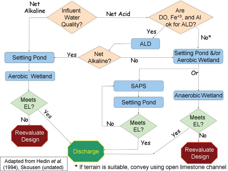
The treatment of net acidic drainage can be handled in a number of ways depending on influent chemistry. If the influent quality is suitable for an ALD, an ALD can be employed as a pretreatment method. A post-ALD settling pond or aerobic wetland is required to allow for the oxidation and precipitation of metals.

Acidic waters that are not suitable for ALDs can be treated with either an anaerobic wetland or a vertical flow system. Due to the potentially large demands on land area of anaerobic wetlands, they are usually only practical for low-flow situations. For systems that receive water that has a pH greater than 4, settling ponds may precede an anaerobic wetland cell to remove significant quantities of Fe. The remaining discharges can be treated using a vertical flow system.

Where terrain is suitable, an open limestone channel can be used to carry the treatment waters while adding additional alkalinity in the process.
Another factor governing system selection will be the cost of available treatment options. Skousen and Ziemkiewicz (2005) have documented cost-effectiveness for a number of different passive system installations by estimating construction costs from system dimensions, assuming 20 year lifetimes, and calculating the cost per ton of acid neutralization using measured performance data. Per-unit acidity treatment costs vary dramatically for all system types. In general, anoxic limestone drains render the most cost-effective passive treatment while open limestone channels were also able to render treatment that was less costly, on average than either type of wetland system and vertical flow systems. Of course, ALDs have very specific influent water quality requirements and are not an option for many AMD discharges, while OLCs can only operate within water conveyances. Generally speaking, the systems that are able to treat the most problematic waters–highly acidic and oxidized–are also the most costly.

Conclusions

Passive treatment systems can be a component of an AMD treatment strategy. They can function as either stand-alone treatment strategies or as pre-treatment to reduce the cost of active treatment. Passive treatment system performance varies significantly among constructed systems, due to differences in site conditions. One factor that influences the performance of systems that utilize limestone is influent acidity, as systems receiving higher acidity are often able to neutralize acidity more effectively. Passive treatment systems are effective at renovating waters with low pH, high acidity, and high concentrations of acid soluble metals including Fe and Al, but their effectiveness at removing Mn is generally limited unless large treatment areas are available.

Acknowledgments

Thanks to Art Rose (Pennsylvania State University) and George Watzlaf (U.S. Department of Energy) for their assistance to the research that supports these recommendations.

References and Literature Cited

Passive Treatment Design Guidelines